Exploring Geospatial Insights with R and rnaturalearth
R
Geo
Author
Aleksei
Published
July 25, 2024
The article showcases the utilization of the rnaturalearth package for handling geographical data. This package provides valuable tools and functions for working with spatial information, making it a powerful resource for data analysts and researchers interested in geographic analyses.
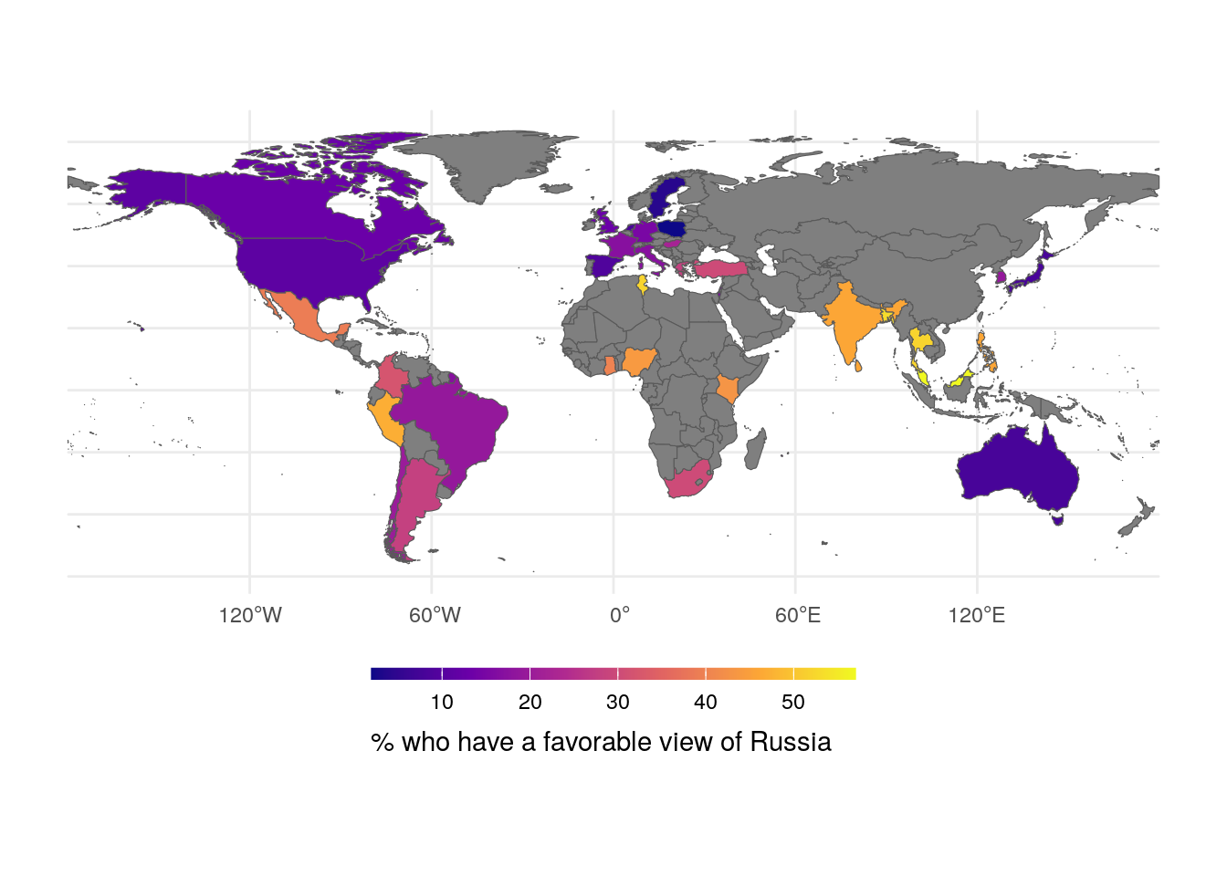
Today, I stumbled upon an article discussing the approval ratings of Russia among people from various nations around the world. As I examined the list, which was sorted from worst to best, a hypothesis formed in my mind: Could the distance between this particular country and others correlate with its citizens’ approval of its international affairs? To explore this, I promptly collected data and calculated the geographical distances between the boundaries of Russia and those of the countries in the list. The null hypothesis posits that distance has no impact on approval rates, while the alternative hypothesis suggests that distance does indeed influence approval levels.
Call:
lm(formula = approval ~ distB, data = df)

Residuals:
    Min      1Q  Median      3Q     Max
-23.345 -11.519  -4.029  13.302  28.339

Coefficients:
            Estimate Std. Error t value Pr(>|t|)
(Intercept)   22.406      3.859   5.806 1.91e-06 ***
distB          1.513      0.814   1.859   0.0723 .
---
Signif. codes:  0 '***' 0.001 '**' 0.01 '*' 0.05 '.' 0.1 ' ' 1

Residual standard error: 16.02 on 32 degrees of freedom
  (1 observation deleted due to missingness)
Multiple R-squared:  0.09743,   Adjusted R-squared:  0.06922
F-statistic: 3.454 on 1 and 32 DF,  p-value: 0.07231
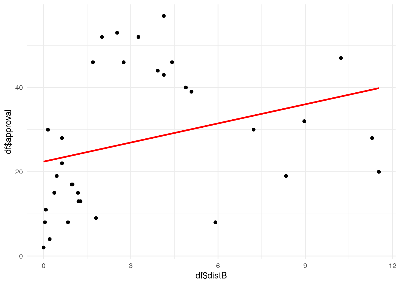
The model explains less than 10% of variability. P-value for distance is 0.072, so the null hypothesis cannot be rejected at the level of 0.05. Scatter plot also shows no obvious trend.
qplot(df$distB, df$approval) +geom_point() +stat_smooth(method ="lm", se = F, color ="red", formula = y ~ x)
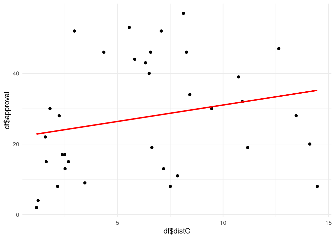
It emerged that the geographical distance between boundaries was statistically insignificant. However, I propose an alternative hypothesis in this scenario. Russia, being an exceptionally vast country, shares proximity with Asian nations in its eastern part. Interestingly, these eastern countries exhibit a more favorable attitude toward Russia compared to their European counterparts. One plausible explanation for this discrepancy is the absence of significant Russian territorial interests in Asia. Since Moscow, the capital, lies in the western part of Russia, let’s measure the distance between capitals and explore this further using regression analysis.
Call:
lm(formula = approval ~ gdp_pc, data = df)

Residuals:
    Min      1Q  Median      3Q     Max
-29.612  -6.029   1.617   4.936  22.483

Coefficients:
            Estimate Std. Error t value Pr(>|t|)
(Intercept) 42.26819    2.63352  16.050  < 2e-16 ***
gdp_pc      -0.67906    0.09049  -7.505 1.52e-08 ***
---
Signif. codes:  0 '***' 0.001 '**' 0.01 '*' 0.05 '.' 0.1 ' ' 1

Residual standard error: 10.15 on 32 degrees of freedom
  (1 observation deleted due to missingness)
Multiple R-squared:  0.6377,    Adjusted R-squared:  0.6264
F-statistic: 56.32 on 1 and 32 DF,  p-value: 1.521e-08
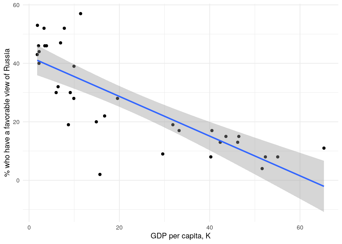
and it yielded promising results. The coefficient associated with GDP showed a remarkably low p-value of 1.52e-08, providing strong evidence against the null hypothesis. The coefficient of determination (R-squared) was also quite favorable at 0.6377, indicating that the model captures a substantial portion of the variation in approval rates. The coefficient with gdp_pc indicates that for every additional thousand USD of GDP per capita, there is a corresponding 0.7 percentage point decrease in the approval rate.
qplot(df$gdp_pc, df$approval) +geom_point() +stat_smooth(method ="lm", formula = y ~ x) +labs(x ="GDP per capita, K", y ="% who have a favorable view of Russia")
In an effort to enhance predictive power, one can explore the possibility of non-linear dependencies. Let’s consider using the logarithm of GDP as a predictor.
model <-lm(approval ~log(gdp_pc), data = df)summary(model)
Call:
lm(formula = approval ~ log(gdp_pc), data = df)

Residuals:
    Min      1Q  Median      3Q     Max
-22.983  -5.332  -0.769   3.175  28.181

Coefficients:
            Estimate Std. Error t value Pr(>|t|)
(Intercept)   58.164      3.828  15.194 3.46e-16 ***
log(gdp_pc)  -12.052      1.371  -8.794 4.77e-10 ***
---
Signif. codes:  0 '***' 0.001 '**' 0.01 '*' 0.05 '.' 0.1 ' ' 1

Residual standard error: 9.125 on 32 degrees of freedom
  (1 observation deleted due to missingness)
Multiple R-squared:  0.7073,    Adjusted R-squared:  0.6982
F-statistic: 77.33 on 1 and 32 DF,  p-value: 4.77e-10
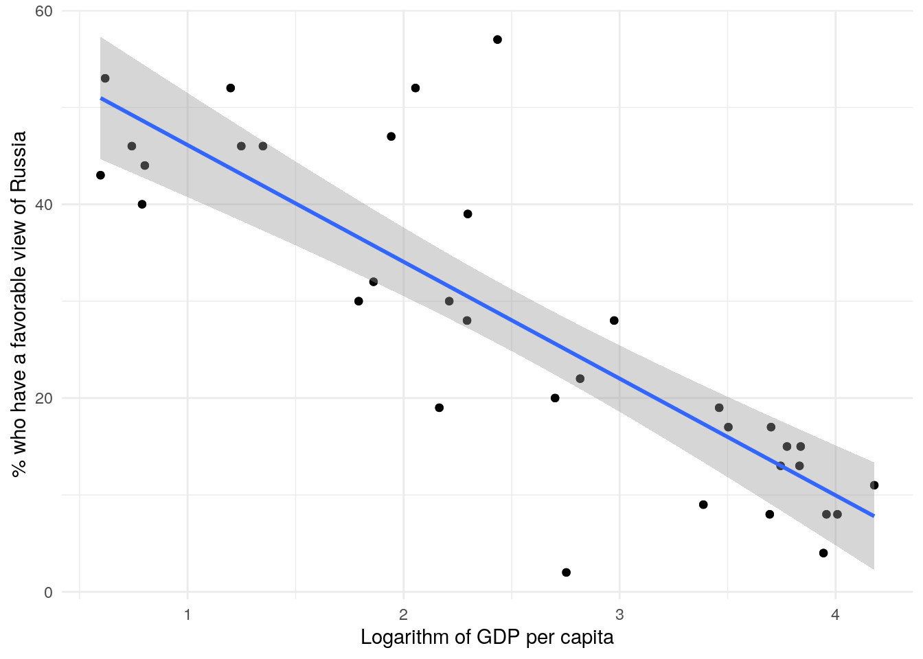
The resulting model yields an impressive R² value of 0.7073, indicating that it explains the vast amount of the variation. Additionally, the p-value of 4.77e-10 provides the strongest evidence against the null hypothesis.
qplot(log(df$gdp_pc), df$approval) +geom_point() +stat_smooth(method ="lm", formula = y ~ x) +labs(x ="Logarithm of GDP per capita", y ="% who have a favorable view of Russia")
However, this improved model is more complex and less straightforward to explain. Allow me to attempt an interpretation: If a country’s GDP per capita is 1% lower than another country’s, it tends to have 0.12% more people who approve of Russia.
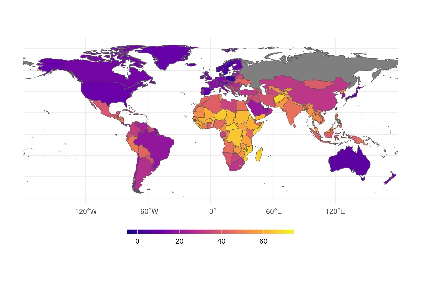
Now that we’ve obtained the regression model, we can use it to make predictions for the remaining countries and visualize the results on a map. By assigning colors based on predicted approval rates, we’ll create an informative and visually appealing representation.